Resolving the PatchGAN Paradox
A critic that got better at judging every local patch made the segmentation worse. Four conditional-GAN discriminators, 369 brain MRI volumes, one generator held fixed — and two failure modes you can predict from the kernel size alone.
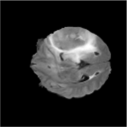
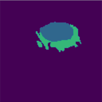
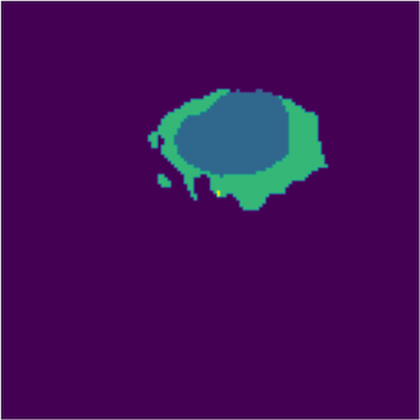
A U-Net hedges. A critic makes it commit.
A 2D U-Net trained on pixel-wise cross-entropy optimises every voxel independently. Faced with an ambiguous boundary voxel — and in glioma annotation almost every boundary voxel is ambiguous — it hedges, predicting the average of the plausible expert answers. The result is the signature failure of CNN segmentation: overly safe, over-smoothed boundaries that blur the line between necrotic core and healthy white matter.
A conditional GAN replaces part of that objective with a second network whose only job is to answer "given this MRI, was this mask drawn by a human?" That is a learned shape prior — something no per-pixel loss can express.
But a discriminator is not one thing. It has a kernel size, a stride, a downsampling strategy and a verdict geometry, and this study finds that two of those choices break it outright.
The research question. What architectural constraints does a PatchGAN discriminator have to satisfy before adversarial supervision helps rather than harms a multi-class medical segmentation model?
Four models, three lessons
Same generator, same data, same 35 epochs. Only the critic changes — and two of the four fail in ways that are diagnosable before training starts.
No critic — baseline U-Net
Pixel-wise cross-entropy only. Segments the tumour reliably and scores 99.27 % pixel accuracy, but produces exactly the smoothed, low-confidence boundaries the study set out to fix.
25.38 dB · SSIM 0.9577 · 88 min
3×3 kernel, stride 2
A 3×3 window advancing 2 pixels at a time does not tile its input evenly: alternating columns are seen twice, then once. That asymmetric overlap imprints checkerboard artefacts straight into the predicted mask.
24.64 dB · SSIM 0.9510 · 148 min
3×3 kernel, stride 1 + MaxPool
The tiling fix works — artefacts vanish and this model reaches the best local segmentation loss in the study, 0.035. Its global structural similarity then collapses to 0.9341, the worst result recorded.
21.62 dB · SSIM 0.9341 · 211 min
4×4 kernel, stride 2
4 divides by 2. Every input column is seen by exactly two windows, so feature extraction is symmetric and no artefacts appear — while the verdict still covers enough of the slice to preserve global anatomy.
25.96 dB · SSIM 0.9583 · 137 min
The clinical pipeline — and the perception–distortion trade-off
Contrast-limited adaptive histogram equalisation makes tumour boundaries visibly crisper to a human reader and improves the segmentation loss, yet PSNR falls 1.2 dB. PSNR and SSIM read a deliberate contrast shift as distortion. Where diagnostic clarity and a distortion metric disagree, the study argues the clinician wins. 24.76 dB · SSIM 0.9582
Why 4 ÷ 2 works and 3 ÷ 2 does not
The whole ablation turns on one integer division. A convolution window of size k advancing by stride s covers each input position a number of times that is constant only when k is a multiple of s.
k=4, s=2 → [2,2,2,2,2,2] against
k=3, s=2 → [2,1,2,1,2,1]. Model C removes the asymmetry a different way
— stride 1 gives uniform coverage of 3 — but pays for it with the paradox.The PatchGAN Paradox
Model C is the most interesting failure in the study because it fails while winning. Replacing strided convolutions with stride-1 convolutions and max-pooling made its discriminator an extremely capable local judge, and the generator's segmentation loss fell to 0.035 — the best figure any model in the ablation achieved. Its global structural similarity fell to 0.9341 — the worst.
The mechanism: the discriminator became so adept at penalising individual patches that the cheapest way for the generator to fool it was to inject high-frequency micro-texture into the mask. Every patch looked convincingly real. The mask as a whole stopped being a continuous anatomical object — the one property radiomics and surgical planning actually depend on.
Local realism and global coherence are separate objectives, and optimising hard for the first actively destroys the second. PatchGAN works for photographic translation because photographic realism is locally determined. A 4-class label map has almost no local information: a patch of pure "edema" is identical whether the mask is perfect or displaced by 40 pixels.
Model C also destabilised the adversarial game outright — its discriminator loss climbed from 9.06 to 12.48 across 35 epochs instead of settling near 1.0. See the divergence in the training curves →
The whole study in one table
| Configuration | Kernel / stride | Artefacts | Seg loss | PSNR (dB) | SSIM | Verdict |
|---|---|---|---|---|---|---|
| Model A — U-Net | n/a | none | 0.0177 | 25.3817 | 0.9577 | over-smoothed baseline |
| Model B — cGAN | 3×3, s2 | checkerboard | 0.0378 | 24.6395 | 0.9510 | structurally flawed |
| Model C — cGAN | 3×3, s1 + pool | none | 0.0355 | 21.6154 | 0.9341 | the PatchGAN Paradox |
| Model D — cGAN | 4×4, s2 | none | 0.0198 | 25.9556 | 0.9583 | the Goldilocks Zone |
| Model D + CLAHE | 4×4, s2 | none | 0.0194 | 24.7633 | 0.9582 | optimal clinical balance |
Every figure is read from a printed cell output in the published notebooks. Where the accompanying paper quotes different values for Model D, the notebook-measured value is used here. See limitations for how tightly these gaps should be read.
What the models actually predict
Unmodified output cells from the notebooks that produced them.
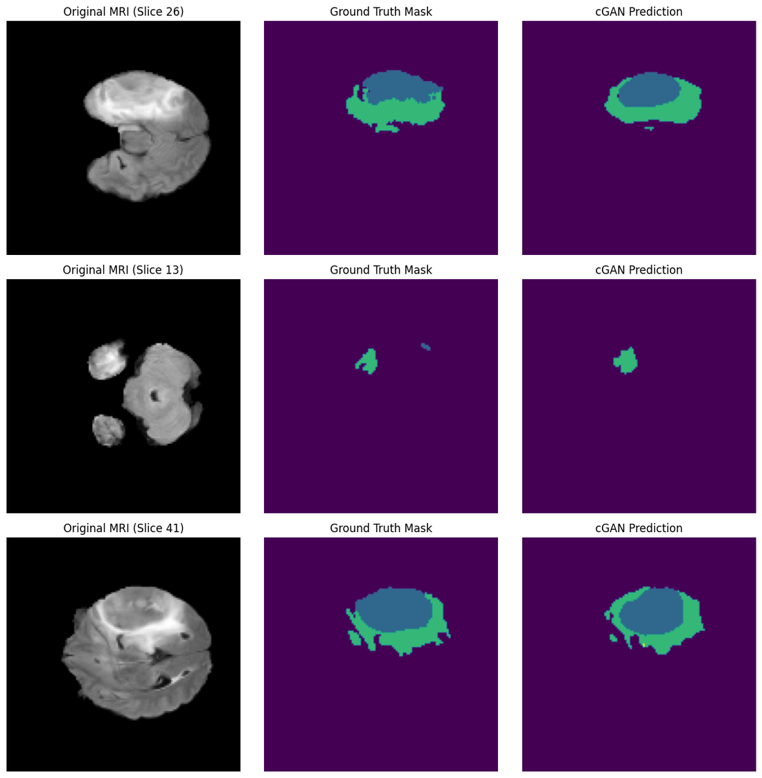


- Necrotic / non-enhancing core
- Peritumoral edema
- GD-enhancing tumour
Go deeper
The study
Purpose, dataset, methodology, the two failure modes, the perception–distortion trade-off, and the limitations in full.
Results
Interactive training curves for all five runs, the complete metric tables and the full prediction gallery.
Notebooks
All eight Kaggle runs rendered in full — code, console output and figures, exactly as they executed.