Architectural Ablation Study of Conditional GANs for MRI Brain Tumour Segmentation
Resolving checkerboard artefacts and the PatchGAN Paradox — a four-stage discriminator ablation on BraTS 2020, with one generator held fixed throughout.
Abstract
Automated brain tumour segmentation from MRI is a critical task in neuro-oncology. Convolutional networks such as the U-Net excel at spatial mapping but, trained on pixel-wise loss alone, produce overly smoothed boundaries that fail to capture the micro-anatomical texture separating a necrotic core from healthy white matter. This study introduces a conditional GAN to enforce high-frequency anatomical realism, and asks what architectural constraints the discriminator must satisfy for that to work.
A four-stage ablation compares a baseline U-Net against three PatchGAN variations, with the generator, data pipeline and epoch budget identical throughout. We show that a 3×3 kernel with a stride of 2 introduces destructive checkerboard artefacts, because the kernel does not divide evenly by the stride. Correcting that with a stride-1 kernel and max-pooling achieves the best local segmentation loss in the study (0.035) but triggers the PatchGAN Paradox: hyper-optimisation for local texture drives global structural similarity down to 0.934, the worst result recorded. A 4×4 PatchGAN with a stride of 2 resolves both failure modes, achieving the best structural agreement with expert masks while keeping boundaries sharp and artefact-free.
Index terms: conditional GAN, brain tumour segmentation, U-Net, PatchGAN, checkerboard artefacts, image enhancement.
1. Purpose of the study
Glioma treatment planning needs more than "is there a tumour". Surgeons and radiation oncologists need the lesion decomposed into three biologically distinct sub-regions, each with different clinical meaning:
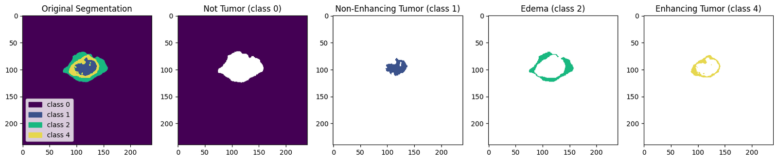
- Necrotic / non-enhancing core — dead tissue at the centre of the lesion.
- Peritumoral edema — swelling in surrounding tissue; defines the radiation margin.
- GD-enhancing tumour — actively proliferating tissue that takes up contrast agent.
Drawing these by hand across 155 axial slices in four MRI sequences takes an expert hours per patient, and inter-rater agreement is imperfect. That variability is itself informative: it means the "correct" boundary is a distribution, not a single answer.
This is exactly where a pixel-wise loss behaves badly. Categorical cross-entropy, faced with an ambiguous boundary voxel, hedges — it predicts the mean of the plausible annotations, which systematically produces the over-smoothed, low-confidence edges characteristic of CNN segmentation. It also has no mechanism to penalise anatomically impossible output: a handful of stray "enhancing tumour" pixels in the cerebellum costs almost nothing in cross-entropy but would be rejected instantly by any radiologist.
A conditional GAN supplies the missing signal. A second network is trained to answer one question — given this MRI, was this mask drawn by a human? — and the generator is trained to fool it. In principle the discriminator learns the statistics of real annotations: connectivity, the core-inside-rim nesting, plausible lesion morphology. That is a shape prior no per-pixel loss can express.
But "a discriminator" is not one design. It has a kernel size, a stride, a downsampling strategy and a verdict geometry — and this study finds that two of those choices break it outright.
Research question. What architectural constraints must a PatchGAN discriminator satisfy before adversarial supervision improves rather than degrades multi-class medical segmentation?
2. Contributions
- A complete 2D segmentation pipeline for BraTS 2020 that trains inside a free Kaggle GPU session: a memory-safe generator streaming one patient volume per step, 99.27 % pixel accuracy and per-class Dice up to 0.708 on 45 held-out patients.
- A conditional-GAN segmentation trainer written from scratch with
tf.GradientTaperather thanmodel.fit(), implementing a composite objective (adversarial BCE + λ·cross-entropy, λ = 100) and updating both networks inside one compiled@tf.functionstep. - A demonstration that kernel/stride divisibility governs artefact formation in the discriminator, with the failure reproduced empirically (Model B) and the fix verified (Model D).
- The identification and naming of the PatchGAN Paradox — a configuration that simultaneously achieves the best local segmentation loss and the worst global structural similarity in the study.
- A perception–distortion analysis of CLAHE preprocessing, showing that a contrast enhancement which improves segmentation loss and clinical readability is penalised by PSNR and SSIM.
- An audit of the evaluation methodology itself, documented in full in §7 rather than quietly corrected.
3. Dataset
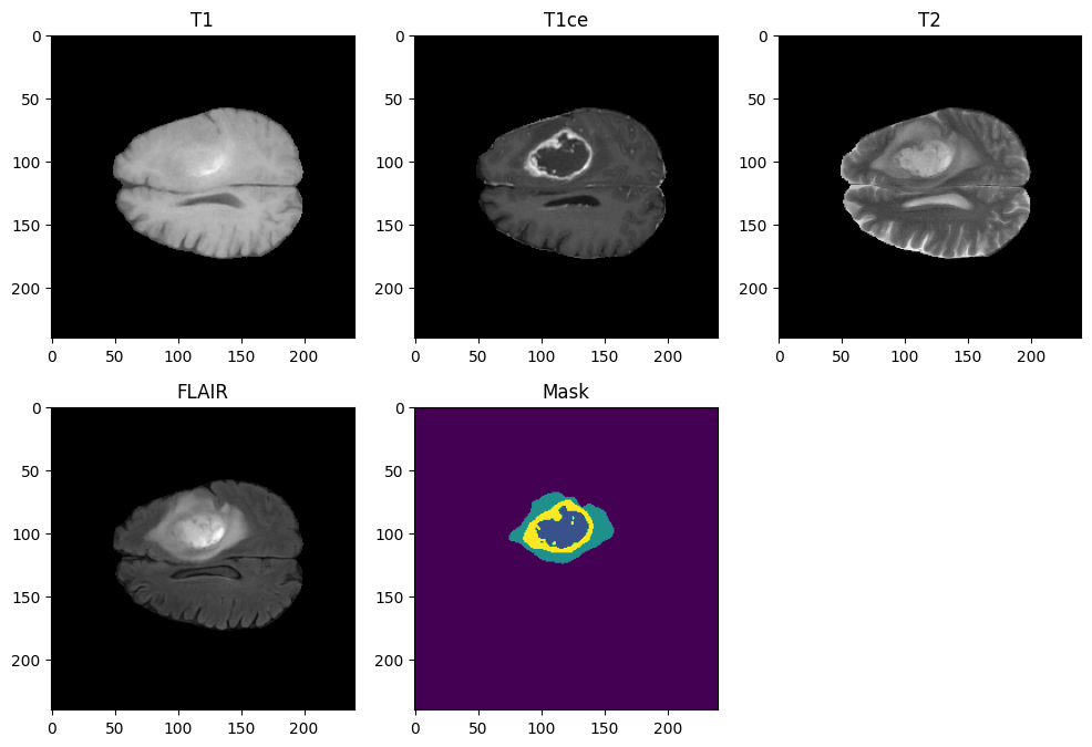
The BraTS 2020 training set: 369 pre-operative multimodal MRI studies of glioma patients, co-registered, skull-stripped, resampled to a 1 mm isotropic grid, with voxel-wise expert consensus annotation.
- Volumes
- 369 patients · 240 × 240 × 155 voxels per sequence
- Sequences
- T1, T1ce (post-contrast), T2, T2-FLAIR
- Labels
- 0 background · 1 necrotic/non-enhancing core · 2 peritumoral edema · 4 GD-enhancing tumour (label 3 unused in this release)
- Format
- NIfTI (
.nii), float64, raw intensities up to ~1855 - Split
- 250 train / 74 validation / 45 test patients (68 / 20 / 12 %)
3.1 Why only two of the four sequences
Feeding all four doubles the input tensor for a marginal information gain, because the pairs are highly correlated. Two were selected on physical grounds:
- T1ce over T1 — gadolinium contrast makes actively proliferating tumour light up, which is precisely the boundary a plain T1 leaves ambiguous.
- T2-FLAIR over T2 — FLAIR suppresses the cerebrospinal-fluid signal that dominates a T2 image, isolating edema against a dark background instead of a bright one.
The result is a 2-channel input whose channels are close to complementary: T1ce carries the core, FLAIR carries the edema.
4. Preprocessing
All five runs share one keras.utils.Sequence data generator, so any difference in
results is attributable to the discriminator and nothing else. Loading all 369 volumes into RAM
would need roughly 100 GB; the generator instead yields one patient at a time and builds the
batch on the fly.
- Load the T1ce and FLAIR NIfTI volumes plus the segmentation for one patient.
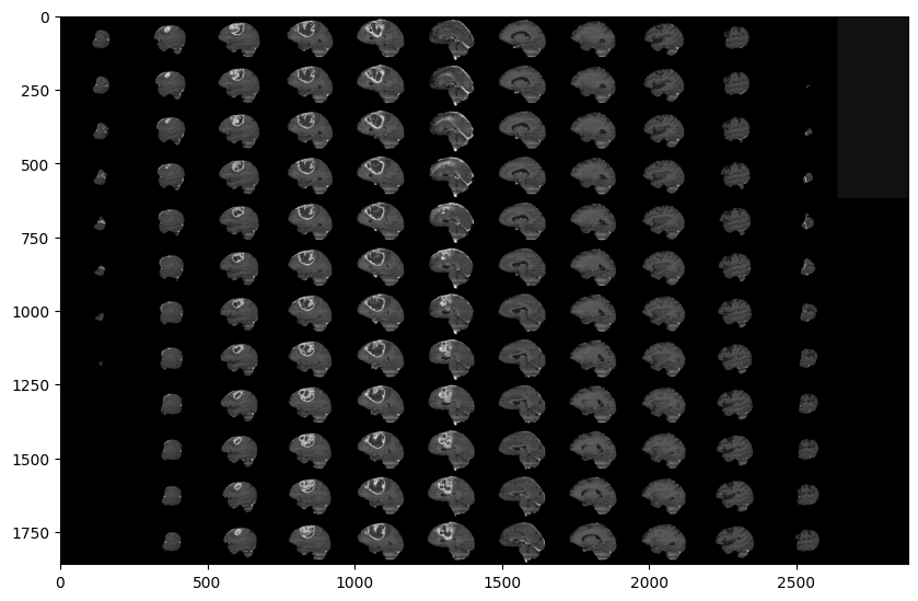
- Slice 100 contiguous axial slices starting at index 22. The first and last ~20 % of a volume is empty space outside the brain and contributes only background.
- Resize each 240×240 slice to 128×128 by bilinear interpolation — a
power of two divides cleanly through four
MaxPooling2Dlevels. - Stack T1ce and FLAIR into the channel axis →
(100, 128, 128, 2). - Remap label 4 → 3 for contiguity, then one-hot encode to
(100, 128, 128, 4). One-hot matters: integer labels would imply "enhancing" is three times "core", an ordering that does not exist. - Normalise by dividing by the volume maximum, guarded against an all-zero volume.
4.1 CLAHE as a pre-training catalyst
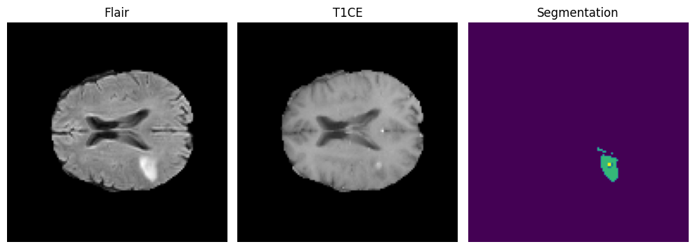
The final pipeline variant adds contrast-limited adaptive histogram equalisation (clip limit 2.0, 8×8 tiles) plus a 3×3 elliptical morphological kernel before the tensor is built. The argument is not cosmetic: CLAHE mathematically amplifies low-contrast boundaries and standardises tissue intensity across scans, which prevents the generator from hallucinating structure in poor-contrast regions. A GAN generator asked to produce a realistic mask where the input carries no signal will invent one; raising local contrast removes the incentive.
A data defect worth recording. One case, BraTS20_Training_355, ships with a
mis-named segmentation file. Rather than let it fail mid-epoch, the pipeline pre-scans every ID
and drops any patient whose _seg.nii is missing — defensive engineering that
prevents a three-hour training run dying at epoch 12.
5. Methodology
5.1 The generator, held fixed
A 2D U-Net with four downsampling levels (32 → 64 → 128 → 256), a 512-filter bottleneck with dropout, and a mirrored decoder concatenating the matching encoder feature map at every level. The head is a 1×1 convolution to four channels with softmax. 7,759,908 parameters, identical across all five runs. Full layer-by-layer breakdown →
5.2 The adversarial objective
The discriminator receives the MRI slice and a mask concatenated along the channel axis (2 + 4 = 6 channels). That conditioning is what makes it a conditional GAN: it never sees a mask without the scan that produced it, so it cannot memorise what plausible masks look like in general — it must judge whether this mask fits this brain.
d_loss = BCE(1, D(mri, real_mask)) + BCE(0, D(mri, G(mri)))
g_loss = BCE(1, D(mri, G(mri))) + LAMBDA * CCE(real_mask, G(mri))    # LAMBDA = 100
λ = 100 is the load-bearing hyperparameter. Unweighted, the adversarial term would
be roughly 50× louder than the segmentation term and the generator would optimise for a
critic-pleasing mask rather than a correct one. Weighted, cross-entropy stays dominant and the
adversarial signal acts as a tie-breaker between pixel-equivalent solutions. Both networks are
updated in one @tf.function step with separate Adam optimisers
(lr 2×10⁻⁴, β1 0.5).
5.3 The four-stage ablation
The variable under test. All discriminators take the same 6-channel input; they differ in kernel size, stride and downsampling strategy.
| Model | Discriminator | Params | Intent |
|---|---|---|---|
| A | none — pixel-wise loss only | — | establish the floor |
| B | 3×3 kernel, stride 2, batch-norm | 1,560,897 | small-kernel patch critic |
| C | 3×3 kernel, stride 1 + MaxPool | 1,559,937 | remove stride artefacts |
| D | 4×4 kernel, stride 2 | 727,489 | even kernel/stride ratio |
5.4 Training configuration
- Epochs
- 35 for every run
- Steps / epoch
- 250 (one patient volume = one step = 100 slices)
- Model A optimiser
- Adam, lr 1×10⁻³, ReduceLROnPlateau (factor 0.2, patience 2, floor 1×10⁻⁶)
- cGAN optimisers
- Two Adam instances, lr 2×10⁻⁴, β1 0.5, no schedule
- Best checkpoint (A)
- epoch 21,
val_loss0.026537 - Total compute
- 732 GPU-minutes (12.2 hours) across all five runs
6. Results and discussion
6.1 The ablation table
| Configuration | Artefacts | Seg loss | PSNR (dB) | SSIM | Verdict |
|---|---|---|---|---|---|
| Model A — baseline U-Net | none | 0.0177 | 25.3817 | 0.9577 | over-smoothed baseline |
| Model B — 3×3, stride 2 | checkerboard | 0.0378 | 24.6395 | 0.9510 | structurally flawed |
| Model C — 3×3, stride 1 | none | 0.0355 | 21.6154 | 0.9341 | the PatchGAN Paradox |
| Model D — 4×4, stride 2 | none | 0.0198 | 25.9556 | 0.9583 | the Goldilocks Zone |
| Model D + CLAHE | none | 0.0194 | 24.7633 | 0.9582 | optimal clinical balance |
Every value is read from a printed cell output in the published notebooks. Where the accompanying paper quotes different figures for Model D, the notebook-measured value is used here.
6.2 The artifact flaw — Model B
A convolution window of size k advancing by stride s covers each input position a
number of times that is constant only when k is a multiple of s. For
k=4, s=2 every interior column is covered exactly twice. For k=3, s=2 the
coverage alternates 2, 1, 2, 1 — a fixed period-2 spatial bias in how strongly each
input column influences the critic's verdict.
The generator learns that rhythm along with the anatomy and stamps it into the predicted mask as checkerboard artefacts. Model B is the worst structural performer among the artefact-free designs, exactly as deep-learning theory predicts — and worse than having no critic at all.
6.3 The PatchGAN Paradox — Model C
Model C removes the asymmetry a different way: stride-1 convolutions give uniform coverage of 3, and downsampling is handled entirely by 2×2 max-pooling. The artefacts disappear, and the generator's segmentation loss falls to 0.035 — the best figure in the study.
Its SSIM falls to 0.9341 — the worst in the study.
The discriminator became so adept at penalising individual local patches that the cheapest way for the generator to fool it was to inject high-frequency micro-texture into the mask. Every patch reads as convincingly real. The mask as a whole stops being a continuous anatomical object — which is the only property that matters for radiomics or surgical planning.
Max-pooling compounds it. It makes the critic locally translation-invariant, discarding exactly the positional information needed to judge whether a mask sits in the right place. The adversarial game never reached equilibrium: Model C's discriminator loss climbed from 9.06 to 12.48 over 35 epochs while the generator kept improving locally. See the divergence →
The lesson. Local realism and global coherence are separate objectives, and optimising hard for the first can actively destroy the second. PatchGAN works for photographic translation because photographic realism is locally determined — skin texture, brick grain, foliage. A 4-class label map has almost no local information: a patch of pure "edema" is identical whether the mask is perfect or displaced by 40 pixels. All the information lives in the global arrangement.
6.4 The Goldilocks Zone — Model D
A 4×4 kernel with stride 2 divides evenly, so feature extraction is symmetric and no checkerboard appears — and its verdict still integrates enough of the slice that the generator cannot buy local realism at the cost of global structure. It records the best PSNR and SSIM in the study while improving boundary sharpness over the critic-free baseline.
The 0.9583 SSIM indicates that generated masks retain the macroscopic integrity a neurosurgeon needs, while adversarial training addresses the boundary blurring that motivated the study.
6.5 The perception–distortion trade-off — CLAHE
Adding CLAHE to Model D improves the segmentation loss (0.0194 against 0.0198) and produces visibly more readable contrast boundaries. PSNR falls 1.2 dB; SSIM is unchanged to four decimal places.
This is not a contradiction, it is the perception–distortion trade-off. CLAHE deliberately forces a stark contrast shift to expose tumour boundaries. PSNR and SSIM are distortion metrics: they measure deviation from a reference and read deliberate enhancement as error. A metric designed to detect compression artefacts is not equipped to reward diagnostic clarity.
The study's position is that in medical imaging, visual perception and diagnostic clarity supersede strict mathematical distortion metrics where the two disagree. Both are reported here and the numbers stand as measured: Model D is the champion on the structural metrics; Model D + CLAHE is the configuration the authors advance for clinical use.
6.6 Clinical implications
Radiomics and surgical planning depend on continuous, highly confident tumour boundaries. The failure modes documented here map directly onto clinical failure modes: checkerboard artefacts corrupt volume measurements; the micro-texture injected under the PatchGAN Paradox fragments a lesion that is anatomically continuous. An architecture can score well on average pixel accuracy and still be clinically unusable, and this ablation shows precisely which architectural decisions cause that.
7. Limitations
Four properties of the setup constrain how far these results generalise. They are listed here rather than buried, because they change how the numbers above should be read.
7.1 The train/test split was never seeded
train_test_split is called without random_state, so each notebook drew a
different partition of the 369 patients. The evidence is in the evaluation output itself:
the number of tumour-bearing validation slices differs between runs — 4,453 for Model A, 4,623
for Model B, 4,524 for Model C. Sub-decibel PSNR gaps therefore sit inside run-to-run split variance.
The 3 dB collapse of Model C does not, and neither does the artefact / no-artefact distinction,
but the Model A to Model D margin should be read as directional.
This is the first thing to fix in any follow-up.
7.2 MeanIoU as configured is invalid
tf.keras.metrics.MeanIoU(num_classes=4) expects integer class indices but is fed
one-hot targets and softmax probabilities. Both are cast to integers internally, collapsing almost
every value to 0 or 1, and the metric degenerates to a constant 0.5 — exactly what the final
evaluation prints. The correct form is
tf.keras.metrics.OneHotMeanIoU(num_classes=4), or an explicit argmax before
the update. No Mean IoU figure from these runs should be used.
7.3 PSNR and SSIM are proxies, not segmentation metrics
Both are computed on argmax label maps with max_val=3.0 — an image whose pixel
values are class indices 0–3. That is defensible as a structural-agreement proxy and is applied
identically to all five models, so the comparison is internally consistent. It is not comparable to
published BraTS results, which report Dice and 95th-percentile Hausdorff distance per sub-region. A
follow-up should evaluate every variant with the same Dice suite already implemented for Model A.
7.4 Architectural and evaluation scope
- 2D, not 3D. Each slice is segmented without inter-slice context, so nothing prevents an implausible jump between adjacent slices of one lesion.
- Downsampled input. 240×240 → 128×128 discards detail that matters most for the small necrotic core — the weakest-scoring class.
- Single run per configuration. No seed averaging, so no confidence intervals.
- No post-processing. Connected-component filtering would lift every model and would specifically target the micro-texture the paradox introduces.
- Dice only for Model A. The cGAN variants were evaluated with PSNR/SSIM only, so a direct Dice comparison against the baseline is not available.
8. Conclusion and future work
cGANs are effective at sharpening medical image segmentation, but architecture selection is critical. This study empirically establishes that 3×3 kernels with even strides introduce destructive checkerboard artefacts; that correcting the flaw with stride-1 pooling yields exceptional local texture accuracy while falling victim to the PatchGAN Paradox; and that a 4×4 PatchGAN with a stride of 2 provides the balance a clinical mask requires.
- Seed the split and re-run. One
random_statemakes the five-model comparison controlled — a one-line change. - Evaluate every variant with Dice and HD95 per sub-region, so results become comparable to the BraTS leaderboard.
- Move to 3D volumetric segmentation. Penalising structural anomalies across the continuous Z axis targets exactly the global-coherence property the paradox showed to be fragile.
- Sweep λ. The adversarial weight was fixed at 100 and never varied; the balance between plausibility and pixel accuracy is the study's own subject.
- Test intermediate verdict scales. If a global verdict beats a 16×16 grid, the useful receptive field may lie between — a 4×4 or 2×2 verdict grid would locate it.
- Federated training across clinics, aggregating weight updates without moving protected health information. See the deployment roadmap →
References
- Ronneberger, O., Fischer, P., Brox, T. (2015). U-Net: Convolutional Networks for Biomedical Image Segmentation. MICCAI.
- Isola, P., Zhu, J.-Y., Zhou, T., Efros, A. (2017). Image-to-Image Translation with Conditional Adversarial Networks (pix2pix, PatchGAN). CVPR.
- Mirza, M., Osindero, S. (2014). Conditional Generative Adversarial Nets.
- Odena, A., Dumoulin, V., Olah, C. (2016). Deconvolution and Checkerboard Artifacts. Distill.
- Blau, Y., Michaeli, T. (2018). The Perception-Distortion Tradeoff. CVPR.
- Menze, B. et al. (2015). The Multimodal Brain Tumor Image Segmentation Benchmark (BRATS). IEEE TMI.
- Bakas, S. et al. (2017). Advancing the Cancer Genome Atlas glioma MRI collections with expert segmentation labels. Scientific Data.
- BraTS 2020 challenge data description, CBICA, University of Pennsylvania.
All figures on this page are outputs of the notebooks listed under Notebooks, and every number is traceable to a printed cell output in one of those runs. This work is a research and educational exercise; it is not a medical device and must not inform clinical decisions.